

How to Calculate OEE: The Manufacturers Complete Guide to Overall Equipment Effectiveness
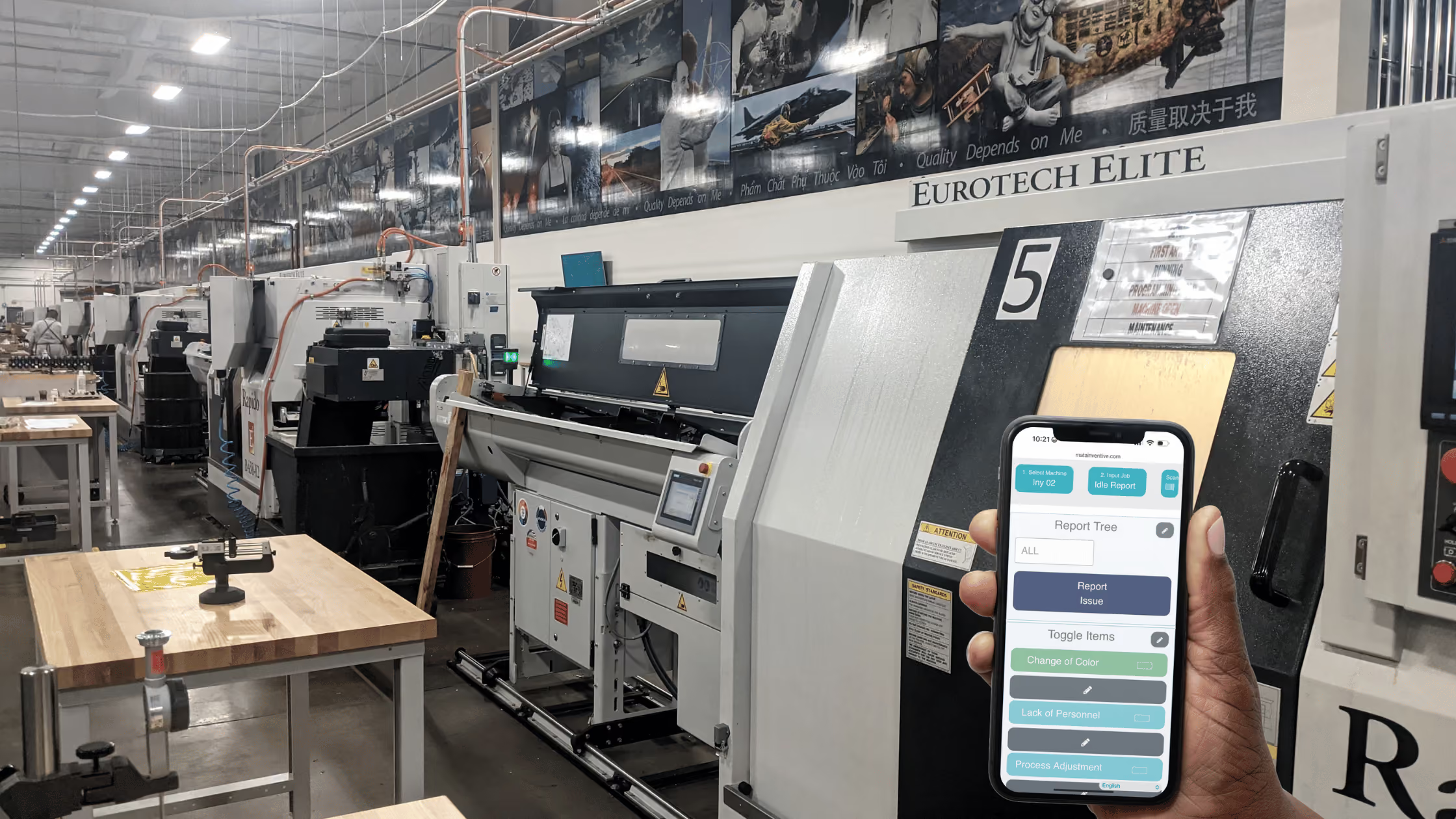
Overall Equipment Effectiveness (OEE) measures the share of planned production time converted into good output at the ideal production rate. Calculate it by multiplying Availability, Performance, and Quality. Reliable OEE requires a defined production schedule, measured run time, an ideal cycle time for the product, and matching total and good part counts.
This guide explains the calculation and the decisions behind it. Use it to establish a baseline, compare shifts fairly, and identify losses that affect capacity, delivery, and cost. For the wider context, start with SensFlo’s Machine Monitoring Guide.
In this guide
- OEE formulas and required inputs
- Measurement rules
- CNC and injection molding examples
- Validation and aggregation
- From OEE losses to production decisions
OEE formulas and the data behind them
Calculate each factor as a decimal, multiply the factors, then multiply the result by 100 to express OEE as a percentage. Keep cycle time and run time in the same units. The underlying formulas follow Vorne’s OEE calculation guidance.
- Availability = Run Time ÷ Planned Production Time.
- Performance = (Ideal Cycle Time × Total Count) ÷ Run Time.
- Quality = Good Count ÷ Total Count.
- OEE = Availability × Performance × Quality.
- For one consistent product rate, OEE also equals (Good Count × Ideal Cycle Time) ÷ Planned Production Time.
| Input | Definition | Source to establish |
|---|---|---|
| Planned production time | Time when the process is intended to produce | Approved shift and production schedule |
| Stop time | Availability loss within planned production time | Timestamped events and defined stop threshold |
| Run time | Planned production time minus stop time | Validated machine state history |
| Ideal cycle time | Fastest achievable time per output unit under optimal conditions | Engineering baseline for the part and process |
| Total count | All units produced within the measurement window | Validated counter or reconciled production record |
| Good count | Units meeting requirements on the first pass | Quality records or confirmed good and reject counts |
All six inputs must describe the same equipment, production window, and output unit. A sensor that detects activity can support Availability, but complete OEE also needs speed and quality information. If a required input is unavailable, report the available metric and identify the missing input. Assuming 100% Quality creates a provisional estimate that should be labeled.
Define measurement rules before comparing OEE
Planned production time and scheduled stops
Begin with shift time and remove periods when there is no intention to produce, such as an excluded break. A scheduled changeover within intended production time remains a production loss under the convention used here. A reason called “planned maintenance” does not automatically remove that event from the denominator. Document the scheduling rule separately from the reason code.
For example, an eight hour shift with a 30 minute break has 450 minutes of planned production time if production is not intended during that break. If the equipment is expected to continue producing while operators rotate through breaks, that same exclusion would be inappropriate. Record the rule once and apply it consistently.
Micro stops, slow cycles, and double counting
Select a stop threshold suited to the process. Under the convention in this guide, longer stops reduce Availability, while short interruptions retained within run time reduce Performance through lower output. Record short events for analysis even when they are assigned to Performance. Apply one accounting rule so the same interruption is not deducted from both factors.
Ideal cycle time, cavities, and first pass quality
Use the ideal achievable production rate for each part and configuration. Keep it separate from a scheduling allowance that includes expected losses. For molding, specify whether the rate is expressed per shot or per piece, and account for active cavities. For quality, count parts requiring rework as a first pass loss even if they later become saleable.
Worked OEE examples for CNC and injection molding
The following examples are hypothetical calculations, not SensFlo customer results. They use defined measurement rules and keep time units consistent.
CNC example: one part per cycle
A CNC machine has 450 planned production minutes after the scheduled break is excluded. Stops total 60 minutes, leaving 390 run minutes. Ideal cycle time is one minute per part. The machine produces 350 parts, of which 343 pass on the first attempt.
| Factor | Calculation | Result |
|---|---|---|
| Availability | 390 ÷ 450 | 86.67% |
| Performance | (1 × 350) ÷ 390 | 89.74% |
| Quality | 343 ÷ 350 | 98.00% |
| OEE | (343 × 1) ÷ 450 | 76.22% |
Good output represents 343 ideal production minutes out of 450 planned minutes. The remaining 107 minutes comprise 60 minutes of stop loss, 40 minutes of speed loss, and seven ideal minutes of quality loss. That breakdown gives the supervisor a practical starting point: investigate the largest stop categories before choosing an improvement project.
Injection molding example: four active cavities
A press has 420 planned production minutes and 45 minutes of stop loss, leaving 375 run minutes. The ideal shot cycle is 30 seconds with four active cavities. The ideal time per piece is therefore 7.5 seconds, or 0.125 minutes. Production totals 700 shots and 2,800 pieces; 2,744 pieces pass first inspection.
| Factor | Calculation | Result |
|---|---|---|
| Availability | 375 ÷ 420 | 89.29% |
| Performance | (0.125 × 2,800) ÷ 375 | 93.33% |
| Quality | 2,744 ÷ 2,800 | 98.00% |
| OEE | (2,744 × 0.125) ÷ 420 | 81.67% |
Multiplying a 30 second shot time by 2,800 pieces would overstate Performance because each shot produces four pieces. If a cavity is blocked during a run, record the configuration change and split the calculation into appropriate segments. This helps the team distinguish a process loss from an incorrect counter or rate setting.
Validate OEE before using it to benchmark production
- Match the start and end times of the schedule, event history, production counts, and quality records.
- Reconcile total count with good count plus first pass rejects or rework. Identify unresolved quality disposition.
- Observe the equipment through production, setup, idle operation, and recovery to verify state definitions.
- Check counter resets, duplicate pulses, missed cycles, and active cavity changes.
- Investigate Performance above 100%. Check the ideal cycle baseline, time units, configuration, and counts.
- Mark gaps in data coverage and separate missing communication from confirmed machine downtime.
For the two examples above, the component calculation and the good output calculation produce the same OEE before rounding. Keep full precision during calculation and round only the displayed result. Disagreement between the two approaches is a useful signal to check the input definitions.
How to aggregate machines and changing products
An arithmetic average of machine percentages gives a short production run the same influence as a full shift. For comparable, independent production segments using this convention, calculate a time weighted OEE as the sum of Good Count × Ideal Time per Unit across segments, divided by the sum of Planned Production Time. Preserve each segment’s appropriate ideal rate.
This aggregate reflects effectiveness against planned equipment time. It does not describe plant throughput automatically. Serial machines can process the same output, and high OEE on a nonconstraint asset may not increase finished goods. Define the reporting scope, publish the weighting method, and retain machine and factor detail behind any summary.
What counts as a good OEE score?
Set targets around comparable equipment, product mix, setup frequency, and measurement rules. An initial baseline helps identify improvement potential. A universal target can mislead when comparing a CNC job shop with frequent setups to a stable, long production run. Review Availability, Performance, and Quality alongside the composite score.
Turn OEE losses into production and financial decisions
Start with the asset limiting delivery or throughput. Review its largest losses, assign an owner, and check whether the intervention changes the relevant factor without creating a quality or safety problem. Improved reporting may initially reveal more losses than the previous logs recorded; establish the validated baseline before claiming an operating gain.
Use automated downtime tracking to develop the event history and reason codes behind Availability. If equipment has no accessible controller data, the legacy machine connectivity guide explains the options and measurements to validate.
Recovered time creates a revenue opportunity when demand, downstream capacity, and staffing allow additional good output. Avoided overtime or scrap can support savings. Calculate those benefits separately and avoid counting the same improvement twice. SensFlo’s ROAI Calculator provides a place to explore your own assumptions.
How FloControl supports the measurement framework
SensFlo FloControl™ organizes machine signals into production visibility, including utilization, downtime, cycle activity, and OEE. Its published connectivity options include sensors, digital and analog inputs, and supported controller protocols. The available measurements depend on the equipment and deployment configuration. Confirm how counts, quality, and scheduled production time will be supplied for your OEE scope.
SensFlo’s Axxis Corporation success story reports a utilization increase of more than 20% within one month. That is evidence of a reported utilization outcome; it should not be relabeled as an OEE increase. Use customer results as context for evaluation while measuring your own baseline.
For platform selection, continue to the machine monitoring software buyer’s guide or SensFlo vs Evocon. Bring your equipment list, calculation rules, and missing inputs to a SensFlo consultation so the proposed scope can be assessed against your production goals.
Frequently Asked Questions
What is the formula for OEE?
OEE equals Availability × Performance × Quality. Calculate the three factors as decimals, multiply them, and express the result as a percentage. For a single consistent product rate, the equivalent formula is Good Count × Ideal Cycle Time ÷ Planned Production Time.
Is OEE the same as machine utilization?
Utilization measures machine use against a defined time base. OEE also includes production speed and first pass quality. State the denominator used for utilization before comparing it with OEE Availability.
Do planned stops reduce OEE?
A planned stop during time when production is intended can reduce Availability. Periods when production is not intended may be excluded from planned production time under a documented scheduling rule. The reason code alone does not determine the denominator.
Can OEE be calculated without quality data?
Complete OEE requires a good count or another validated first pass quality input. An estimate assuming 100% Quality must be labeled provisional. Availability and Performance can still be reported separately while quality data is established.
How do you calculate OEE for a multicavity mold?
Use consistent output units. Divide ideal shot cycle time by the number of active cavities to obtain ideal time per piece, then use piece counts for Performance and Quality. Segment the run when the active cavity configuration changes.
Why can OEE Performance exceed 100%?
Under an ideal achievable cycle baseline, Performance above 100% indicates that the inputs or baseline need review. Common causes include an overly slow ideal cycle setting, inconsistent units, duplicate counts, and incorrect cavity configuration.
You might also like...



Talk to us
Let us take your company to the next level. Let’s have a chat and find out how we can help you.

