¿Cómo calcular y mejorar el aprovechamiento de maquinaria con sensores IoT?

Key takeaway
Machine utilization is the share of available time a machine actually runs, calculated as actual operating time ÷ total available time × 100. To see the full effectiveness picture, multiply Availability × Performance × Quality for OEE. IoT sensors capture the underlying run, idle, and stop data automatically, removing the guesswork and delay that make manual tracking unreliable.
In this guide: the machine utilization formula and how it relates to OEE, a step-by-step walkthrough of Availability, Performance, and Quality, worked examples from metalworking, plastics, food and beverage, and textile production, a manual vs. IoT comparison table, and practical steps to raise utilization once you can measure it.
What Is Machine Utilization, and How Is It Different From OEE?
Machine utilization is the percentage of scheduled time a machine is actually operating, found by dividing actual operating time by total available time and multiplying by 100. OEE goes one layer deeper by combining three factors — Availability, Performance, and Quality — so it accounts for speed losses and defects, not only raw uptime.
Utilization is the simpler of the two metrics and a sensible first step for any shop new to monitoring, because it answers a single direct question: of the hours this machine is staffed and expected to run, how many is it genuinely producing? According to NCD's guide on machine utilization, the core calculation is straightforward, and the real difficulty has always been collecting accurate runtime, downtime, and idle-time data rather than running the math.
The two metrics measure different things and shouldn't be used interchangeably. As CNC Optimization explains, utilization tracks only the proportion of scheduled time the spindle is actively cutting, while OEE multiplies availability, performance efficiency, and quality yield — a shop running 90% availability, 85% performance, and 98% quality lands at roughly 75% OEE, a figure considered world-class in most discrete manufacturing.
How Do You Calculate Availability?
Availability is the percentage of planned production time that a machine is actually running. You calculate it by subtracting all downtime from planned production time, then dividing the result by planned production time. It captures both planned stops like changeovers and unplanned ones like breakdowns or material shortages.
Availability = (Planned Production Time − Downtime) ÷ Planned Production Time
For a worked example, Oxmaint's OEE breakdown uses a CNC cell on an 8-hour shift: 480 planned minutes with 60 minutes of downtime leaves 420 minutes of run time, for an Availability of 87.5%. In machining environments the biggest availability losses are rarely dramatic breakdowns. They are the accumulated minutes between cycles — waiting for material, swapping fixtures, and hunting for tooling — which is exactly the time that no operator stops to log.
How Do You Calculate Performance?
Performance measures how close a machine runs to its ideal speed while it is operating. You calculate it by comparing actual output against the theoretical maximum for the run time available, or equivalently by measuring actual cycle time against the ideal cycle time. It captures reduced speed, idling, and minor stoppages.
Performance is usually the hardest loss to see. As the TeepTrak OEE guide notes, minor stoppages of around 30 seconds each are rarely logged in a production system, yet they can quietly pull Performance from 95% down to 80% across a single shift. These micro-stops are precisely the events that machine-connected monitoring detects automatically and that manual reporting almost always misses.
How Do You Calculate Quality?
Quality is the percentage of good units out of total units produced, found by dividing good parts by total parts. Every scrapped or reworked unit consumed machine time without delivering value, so quality losses cost capacity twice: once for the wasted run time and again for the rework that follows.
Quality = Good Units ÷ Total Units Produced
Quality is the most demanding component in absolute terms. Tractian's analysis of world-class OEE points out that the 99.9% quality target is unforgiving in high-volume settings, where even a 0.5% defect rate can mean thousands of rejected units per shift. Defects also cluster after changeovers and during startup, before a process stabilizes, which is why first-pass yield and scrap rate are the two metrics worth watching most closely.
How Do You Combine the Three Into an OEE Score?
OEE is the product of all three factors: Availability × Performance × Quality. Because they multiply, strong individual scores still compound into a much lower total — 90% in each component yields just 73% OEE. One weak factor pulls the whole result down, which is what makes OEE such a revealing single number.
OEE = Availability × Performance × Quality
The benchmarks give that number meaning. According to the TeepTrak guide, 85% is treated as world-class, 60% is roughly typical, and most manufacturers measure somewhere between 40% and 65% when they first start tracking. Guidewheel adds the important caveat that context decides the right target: a highly automated automotive line can push into the 90s, while a job shop with frequent changeovers and high product mix will naturally run lower and should benchmark against itself.
What Does OEE Look Like in Real Manufacturing?
OEE is a ratio, so it applies to any process — parts, weight, or length — which is why it works across very different shop floors. The clearest way to understand it is through concrete examples from the verticals where machine monitoring delivers the fastest return.
Metalworking
A CNC spindle that looks busier than it is
In an 8-hour shift of 480 minutes, suppose operators spend 45 minutes on breaks, 90 on setup and changeover, 20 loading parts, and 30 on a tool breakage. The spindle is only cutting for 295 minutes, a utilization of 61.4%. CNC Optimization notes that on a $150-per-hour machine, that idle time represents roughly $78,000 in lost revenue a year on a single shift — capacity recoverable without buying equipment. Monitoring it is the first step many metalworking shops take.
Plastics
Injection molding measured in parts, extrusion in kilograms
An injection molding machine with a 4-cavity mold running a 30-second cycle could produce 3,840 mouldings in an 8-hour shift. If it actually makes 3,456 good parts, OEE is 90%, per InTouch Monitoring. The same source shows extrusion measured by weight: a line rated at 450 kg/hr that produces 2,340 kg over an 8-hour shift achieves 65% OEE. Both calculations depend on capturing real cycle and output data, which is where sensors help plastics and molding operations.
Food & Beverage
Changeovers and CIP dominate the losses
World-class OEE in food and beverage typically sits around 82–85% on dedicated high-volume lines, yet many plants run between 40% and 65%, according to Oxmaint's food and beverage analysis. The dominant drains are SKU changeovers, allergen flushes, and clean-in-place cycles. The same analysis reports that cutting changeover duration by 25% typically lifts OEE by 4 to 7 points on high-mix lines — a meaningful gain for any food and beverage operation.
Textiles
Continuous output measured by length
Continuous processes are measured the same way, just in different units. InTouch Monitoring illustrates this with a wire-drawing line running at 300 m/min: over a 12-hour shift it could produce 216,000 metres, so drawing 138,240 metres works out to 64% OEE. The identical length-based logic applies to spinning, weaving, and finishing equipment, where micro-stops and speed losses are the quiet costs that monitoring surfaces for textile production.
Manual vs. IoT-Driven Utilization Tracking: What's the Difference?
Manual tracking relies on operators recording stops and run times by hand, which introduces gaps, delay, and bias. IoT-driven tracking reads machine state directly and continuously, so the data is both more accurate and immediately available. The difference shows up most in the losses humans never log.
The size of that gap is well documented. Machine Tracking describes a 15-machine job shop where the owner estimated utilization at 70–75% from scheduler projections and floor observation; once automatic machine-state capture was deployed, actual spindle-on time across the floor averaged 51%. The missing 20-plus points came from unlogged tool-change delays, operator pauses no one recorded, and between-job idle periods the scheduler had assumed were negligible.
Comparison of utilization tracking methods across accuracy, latency, and setupTracking MethodOEE AccuracyData LatencySetup ComplexityBest ForManual loggingLow — depends on operator diligence; micro-stops and idle gaps routinely missedHigh — entered after the fact, often per shift or per dayLow — paper sheets or spreadsheets, no hardwareVery small shops or a short-term baseline before automatingPLC-only systemsMedium–High — accurate where controllers are accessible and standardizedLow — near real-time from the control systemHigh — requires control-system access, integration, and programming per machineNewer, uniform equipment fleets with in-house controls expertiseIoT sensor platform (FloControl™)High — captures run, idle, stop, and cycle data automatically, including the micro-stops manual methods missReal-time — continuous streaming and instant alertsLow — sensors attach in under 60 seconds, no wiring or controller accessMixed-age, multi-vendor fleets that need fast, plant-wide visibility
Setup time and "no wiring" claims reflect SensFlo FloControl™ deployment data; accuracy and latency characteristics are general to each tracking category.
How Do IoT Sensors Automate Utilization Tracking?
IoT sensors detect machine state through signals such as vibration, current draw, or cycle pulses, then transmit that data wirelessly to a central platform that converts it into utilization, downtime, and cycle-time metrics in real time. Because they read signals directly, they avoid both the wiring of PLC integration and the gaps of manual logging.
The data flow is consistent across platforms. Caddis Systems describes the standard pipeline: an edge device or sensor captures cycle start and stop events, spindle state, alarm codes, and part counts, which a monitoring platform turns into a live feed of which machines are running, which are idle, how long each cycle takes, and why equipment stops. SensFlo's FloControl™ platform follows this model, attaching to any machine in under a minute and surfacing losses most teams discover within their first 30 days.
How Do You Improve Machine Utilization Once You're Measuring It?
Improving utilization starts with attacking the largest loss categories first, not chasing a headline benchmark. The Six Big Losses framework from Total Productive Maintenance groups every loss into breakdowns, setups, minor stops, speed losses, startup defects, and production defects, so each gets the right countermeasure.
Once losses are visible, the gains follow a predictable order. JITbase suggests establishing a 2-to-4-week baseline, expecting shop averages of 30–60% OEE, and targeting a 10-to-20 percentage-point improvement over 6 to 12 months by running a Pareto analysis on downtime and applying SMED to changeovers. The largest single opportunity in most plants is the idle time between jobs that never appears in any report, which is why continuous measurement does more than describe the problem — it makes the recoverable hours actionable. For a quick estimate of what that recovery is worth in your operation, SensFlo's ROAI calculator models the revenue tied to a utilization gain.
The financial stakes explain the urgency. Aggregated downtime research citando el informe 'El verdadero costo del tiempo de inactividad' de Siemens, sitúa las pérdidas combinadas de los 500 fabricantes más grandes del mundo en cerca de 1.4 billones de dólares al año, aproximadamente el 11% de sus ingresos, con un costo promedio en la manufactura de alrededor de 260,000 dólares por hora y una planta típica perdiendo aproximadamente 800 horas de producción anualmente. Gran parte de esto es recuperable en el equipo existente una vez que se tienen los datos para identificarlo.
Preguntas frecuentes sobre la utilización de maquinaria y el OEE
¿Cuál es una buena tasa de utilización de maquinaria?
Una buena tasa depende del modelo de producción. Las líneas dedicadas de alto volumen a menudo superan el 80%, mientras que los talleres de producción variada suelen operar entre el 40% y el 65%. Específicamente para el OEE, el 85% es el punto de referencia de clase mundial ampliamente citado, y la mayoría de los fabricantes comienzan en el rango del 40-65% cuando miden por primera vez. La comparación útil es con tu propia industria y la complejidad del producto, en lugar de un número universal único.
¿Cuál es la diferencia entre la utilización de maquinaria y el OEE?
La utilización de maquinaria mide la proporción del tiempo programado en que el equipo está realmente funcionando — tiempo de operación real dividido por el tiempo total disponible. El OEE va más allá al multiplicar la Disponibilidad, el Rendimiento y la Calidad, por lo que captura las pérdidas de velocidad y los defectos además del tiempo de actividad bruto. La utilización es la métrica inicial más sencilla y un buen punto de partida; el OEE es la imagen completa de la efectividad que muestra dónde se concentran las pérdidas.
¿Cómo miden los sensores IoT la utilización de maquinaria sin cableado?
Los sensores IoT leen el estado de la máquina a partir de señales como vibración, consumo de corriente o pulsos de ciclo, y luego lo transmiten de forma inalámbrica a una plataforma central. Debido a que detectan estas señales directamente en lugar de acceder al sistema de control, se instalan en menos de un minuto y capturan automáticamente el tiempo de funcionamiento, el tiempo de inactividad y las paradas — incluyendo las paradas cortas y los lapsos entre trabajos que el registro manual suele pasar por alto.
¿Qué tan rápido puede el monitoreo IoT mejorar la utilización?
La mayoría de las plantas ven ganancias medibles dentro de los primeros 30 a 90 días. La mejora temprana suele provenir de hacer visible el tiempo de inactividad oculto: cambios de herramientas no registrados, lapsos entre trabajos y microparadas que nunca llegaron a un informe. Los talleres que actúan sobre estos datos suelen apuntar a una ganancia de OEE de 10 a 20 puntos porcentuales en un período de 6 a 12 meses, a menudo sin añadir equipo ni personal.
¿Se puede calcular el OEE en un taller de producción variada?
Sí. La fórmula del OEE se aplica a cualquier proceso, pero el objetivo de clase mundial del 85% fue diseñado para líneas dedicadas de un solo producto y es la meta equivocada para un taller que maneja muchas referencias de piezas en máquinas compartidas. En entornos de alta mezcla, un objetivo del 75-80% es más realista, y la prioridad es reducir las pérdidas por cambio de formato y configuración en lugar de perseguir el punto de referencia principal.
¿Cuánto cuesta el tiempo de inactividad no planificado a los fabricantes?
Las estimaciones varían según el sector y el estudio. Siemens sitúa las pérdidas combinadas para los 500 fabricantes más grandes del mundo cerca de 1.4 billones de dólares al año, aproximadamente el 11% de los ingresos. La investigación de Aberdeen sitúa el promedio de fabricación en alrededor de 260,000 dólares por hora, y la planta típica pierde aproximadamente 800 horas de producción anualmente — gran parte de ello debido a paradas que el monitoreo continuo podría haber detectado antes.
Hablemos
Queremos llevar tu empresa al siguiente nivel. Conversemos para ver cómo podemos ayudarte.
Correo electrónico
info@sensflo.aiTeléfono:
+1 (415) 622-5692Dirección:
21300 Victory Blvd #300, Woodland Hills, CA 91367, Estados Unidos